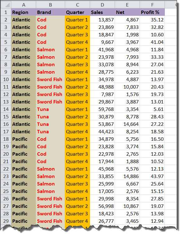
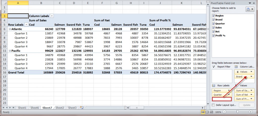
Here is a sample table representing the imaginary Atlantic and Pacific region sales of a fictitious fish company.
(Click to enlarge the images)
As you can see, it’s not easy to look at this data and answer a simple question like “which fish brand is more profitable in Atlantic region?”, or, “Which fish is more profitable in Quarter 2, regardless of region?”
Such “trick questions” is easy to answer when you re-format your data as a Pivot Table.
(1) Select your table.
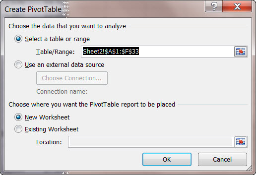
(2) Go to Insert tab on the ribbon and click the PivotTable button on the Tables pod. Create Pivot Table dialog box will display:
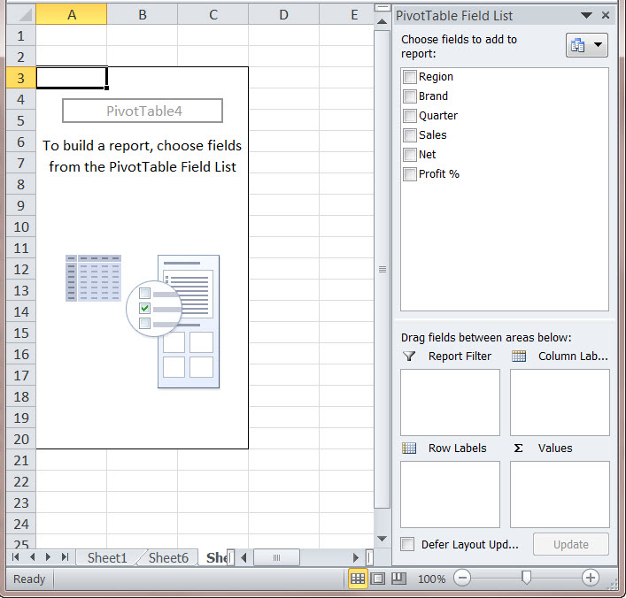
(3) Use the default “New Worksheet” setting and click OK to display the Pivot Table wizard in a new worksheet:
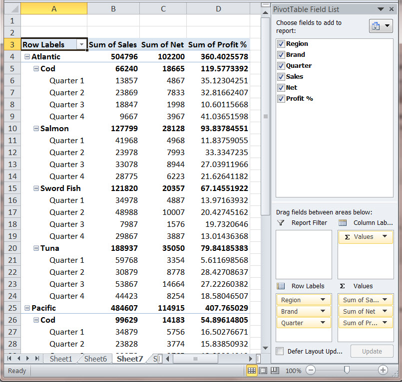
(4) Select the fields (variables) you’d like to include in your Pivot Table by putting a check mark next to them. REMEMBER: Your original data remains intact no matter what you do with your Pivot Table. However, it’s always good practice to keep a backup copy of all your important data before manipulating them.
Your screen now should look something like this:
(5) Now you can click and drag the BRAND field from the ROW labels to the COLUMN labels to create a different Pivot Table:
(6) Now click and drag the QUARTER field from the ROW label to the COLUMN label and drag the BRAND label back to the ROW labels to create yet another Pivot Table:
As you can see, different Pivot Tables display different relationships between selected data, which is the whole idea to this exercise.
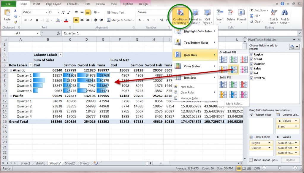
To make these relationships easily detectable, you can select the part of the table that interests you and then switch on different visualization options from HOME Tab > CONDITIONAL FORMATTING. Here is one such example:
